算法为王系列文章,涵盖了计算机算法,数据挖掘(机器学习)算法,统计算法,金融算法等的多种跨学科算法组合。在大数据时代的背景下,算法已经成为了金字塔顶的明星。一个好的算法可以创造一个伟大帝国,就像Google。
算法为王的时代正式到来….
关于作者:
- 张丹, 分析师/程序员/Quant: R,Java,Nodejs
- blog: http://blog.fens.me
- email: bsspirit@gmail.com
转载请注明出处:
http://blog.fens.me/r-epimodel
前言
在上一篇文章 用R语言解读传染病模型 中,我们已经了解传染病动力学模型的背景知识,并且用R语言手动把基本的传染病模型公式进行了编程实现。对于传染病学科中,已经有专业的团队开发出了专业的模型,所以其实我们不需要手动从头写代码,站在巨人的肩膀前进会让我们进步的更快。
本次将介绍的 EpiModel 包就是一个专业做传染病动力学模型的工具,不仅支持基本的SI, SIS, SIR模型,还支持扩展,自定义开发等酷炫功能,让我们进行传染病的模型开发和模拟,有非常大的帮助。
用R进行跨界建模,打破自己的知识壁垒。世界真奇妙,让我们用R来探索吧。
目录
- EpiModel包介绍
- 确定性间隔模型的核心函数
- SI模型实现
- SIS模型实现
- SIR模型实现
- SEIR模型实现
- 基于SI模型实现组间交叉传染
- 网络模型实现
1. EpiModel包介绍
EpiModel 提供了用于模拟和分析传染病动力学数学模型的工具,支持的流行病模型类包括确定性隔间模型、随机个体接触模型和随机网络模型。疾病类型包括有人口统计的 SI、SIR 和 SIS 流行病,可实现自定义可扩展的和模拟任意复杂性的流行病模型。EpiModel中 特有的网络模型,基于在 R 的 Statnet 软件套件中实现的时间指数随机图模型 (ERGM) 的统计框架。
官方网站: http://www.epimodel.org/index.html
EpiModel包整体架构

EpiModel包,支持三类流行病模型提供功能:
- 确定性隔间模型(Deterministic Compartmental Models):模型是确定性的,时间是连续的,解是输入参数和初始条件的固定数学函数,在疾病和人口过渡过程中没有随机变异性。
- 随机个体接触模型(Stochastic Individual Contact Models):参数是随机抽取,其中控制状态间转移的所有比率和风险都是随机抽取的,它们来自由这些比率或概率总结的分布,包括正态分布、泊松分布和二项分布。时间是离散的,ICMs是在离散时间内模拟的,而DCMs是在连续时间内模拟的。
- 随机网络模型(Stochastic Network Models): 两个节点之间连边与否不再是确定的事情,而是根据一个概率决定。网络动力学和疾病传播动力学,这两个动态过程是被视为独立的或者相互依赖的。独立的网络模型假设疾病模拟对时间网络的结构没有影响,尽管时间网络的结构肯定会影响疾病。依赖网络模型允许流行病学和人口统计过程影响网络结构。
EpiModel包,默认支持三种传染病类型,同时允许使用者自己扩展模型内核计算,本文介绍的SEIR模型,就是基于自定模块按公式自己开发的。
- SI:Susceptible-Infective,一种两种状态的疾病,其中存在终生感染而无法恢复。 HIV/AIDS 就是一个例子,尽管在这种情况下,通常将感染阶段建模为单独的隔间。
- SIR:Susceptible-Infective-Removed,一种三期疾病,感染后可终生恢复并产生免疫力。麻疹就是一个例子,但该疾病的现代模型也需要考虑人群中的疫苗接种模式。
- SIS:Susceptible-Infective- Susceptible,一种两阶段疾病,其中一个人可能在一生中从易感状态到受感染状态来回转换。例子包括细菌性性传播疾病,如淋病。
EpiModel包框架下,不仅提供了丰富的功能,有很好的扩展性,还支持自定模型的开发,允许多种状态的设计,支持确定计算的和随机的计算,可模拟真实的传染病传播过程。
2. 确定性间隔模型的核心函数
本文中SI,SIS,SIR,SEIR都是基于确定性间隔模型实现的,因此需要重点了解一下确定性间隔模型的核心函数。
主要有4个:
- param.dcm(),用于设置确定性隔间模型传播参数
- init.dcm(),用于设置确定性隔间模型的人数相关的初始条件
- control.dcm(),用于设置确定性隔间模型的控制参数
- dcm(),加载参数变量,运行模型
查看 param.dcm() 函数定义
> param.dcm
function (inf.prob, inter.eff, inter.start, act.rate, rec.rate,
a.rate, ds.rate, di.rate, dr.rate, inf.prob.g2, act.rate.g2,
rec.rate.g2, a.rate.g2, ds.rate.g2, di.rate.g2, dr.rate.g2,
balance, ...)
参数列表: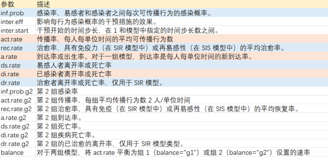
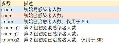
查看 init.dcm() 函数定义
> init.dcm
function (s.num, i.num, r.num, s.num.g2, i.num.g2, r.num.g2, ...)
3. SI模型实现
本文将直接介绍使用EpiModel包的具体实现,关于SI,SIS,SIR模型的具体数据公式和解释,请参考文章:用R语言解读传染病模型
安装和加载EpiModel包
# 安装EpiModel包
> install.packages("EpiModel")

# 加载EpiModel包,并设定运行目录
> library(EpiModel)
> setwd("C:/work/R/covid19")
构建SI模型:初始:日感染率 inf.prob=0.5,日传播率 act.rate=0.5。初始易感染者s.num=500,初始已感染者i.num=1,观察周期nsteps=100。
# 设置模型传播参数
> param <- param.dcm(inf.prob = 0.5, act.rate = 0.5)

# 设置模型人群参数
> init <- init.dcm(s.num = 500, i.num = 1)

# 设置使用SI模型和观察周期
> control <- control.dcm(type = "SI", nsteps = 100)
在param.dcm()函数中,把传染率拆分成了2个值inf.prob和 act.rate,从源代码中这两个参数相乘就是日感染率,这里是给我们提供了一个额外的调解参数,并没有改变模型本身的算法。
运行模型,并查看模型计算结果。查看mod变量,会打印SI模型所有运行参数。
# 运行模型
> mod <- dcm(param, init, control)
> mod
EpiModel Simulation
=======================
Model class: dcm

Simulation Summary
-----------------------
Model type: SI
No. runs: 1
No. time steps: 100
No. groups: 1

Model Parameters
-----------------------
inf.prob = 0.5
act.rate = 0.5

Model Output
-----------------------
Variables: s.num i.num si.flow num
模型结果,可视化输出,直接使用plot()函数即可。
> plot(mod)

上图中,蓝色线为易感染人数,红色线为已感染人数,从图中我们能看到人群的变化过程。
查看模型结果数据集,前10条计算结果,可以直接把mod 转型为data.frame类型,来查看每一个周期的运行结果。
> head(as.data.frame(mod),10)
   time    s.num    i.num   si.flow num
1     1 500.0000 1.000000 0.2832895 501
2     2 499.7167 1.283290 0.3632782 501
3     3 499.3534 1.646568 0.4656817 501
4     4 498.8878 2.112249 0.5966712 501
5     5 498.2911 2.708921 0.7640466 501
6     6 497.5270 3.472967 0.9776201 501
7     7 496.5494 4.450587 1.2496619 501
8     8 495.2998 5.700249 1.5953944 501
9     9 493.7044 7.295644 2.0335064 501
10   10 491.6708 9.329150 2.5866250 501
如果想查看第20个观察周期的传播率、易感染者人数和已感染者人数时,可以使用comp_plot()进行画图,把这一时刻的传播关系可视化展示。
> comp_plot(mod, at = 20, digits = 2)
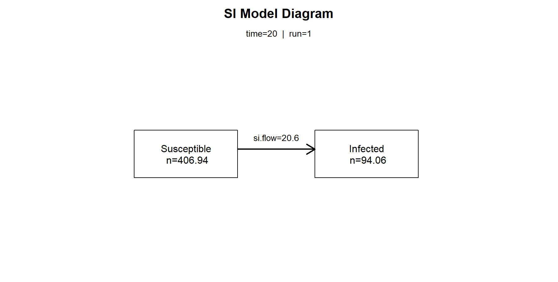
如果想查看第20个观察周期的具体的计算数值时,可以使用summary()函数,指定at=20来看模型的明细数据。
> summary(mod, at = 20)
EpiModel Summary
=======================
Model class: dcm

Simulation Summary
-----------------------
Model type: SI
No. runs: 1
No. time steps:
No. groups: 1

Model Statistics
------------------------------
Time: 20	 Run: 1
------------------------------
                n    pct
Suscept.  406.938  0.812
Infect.    94.062  0.188
Total     501.000  1.000
S -> I     20.601     NA
------------------------------
通过EpiMdoel包来计算SI模型的模拟运行,是非常方便的,省去了我们原来自定义微分方程的过程,而且EpiModel还集成是可视化图、传播链图,参数多样化等高级特性,让我们做传染病的模拟,仅需要几行代码就可以实现。
4. SIR模型实现
通过 SIR模型,进行人口分析。在易感-感染-恢复 (SIR) 模型中,受感染的个体从疾病转变为终生恢复状态,在这种状态下他们将不再易感。
初始:日感染率inf.prob=0.2,日传播率 act.rate=1,恢复率rec.rate=1/20, 出生率a.rate=1/95,死亡率ds.rate=1/100,疾病死亡率 di.rate=1/80, 恢复率dr.rate=1/100。易感染者s.num=1000,已感染者i.num=1,治愈r.num=0,观察周期nsteps=500。
# 设置模型传播参数
> param <- param.dcm(inf.prob = 0.2, act.rate = 1, rec.rate = 1/20,
+                    a.rate = 1/95, ds.rate = 1/100, di.rate = 1/80,  r.rate = 1/100)

# 设置模型人群参数
> init <- init.dcm(s.num = 1000, i.num = 1, r.num = 0)

# 设置使用SIR模型、观察周期、间隔步长
> control <- control.dcm(type = "SIR", nsteps = 500, dt = 0.5)
运行模型,并查看模型计算结果
# 运行模型
> mod <- dcm(param, init, control)
> mod
EpiModel Simulation
=======================
Model class: dcm

Simulation Summary
-----------------------
Model type: SIR
No. runs: 1
No. time steps: 500
No. groups: 1

Model Parameters
-----------------------
inf.prob = 0.2
act.rate = 1
rec.rate = 0.05
a.rate = 0.01052632
ds.rate = 0.01
di.rate = 0.0125
dr.rate = 0.01

Model Output
-----------------------
Variables: s.num i.num r.num si.flow ir.flow a.flow
ds.flow di.flow dr.flow num
模型结果,可视化输出
> par(mar = c(3.2, 3, 2, 1), mgp = c(2, 1, 0), mfrow = c(1, 2))
> plot(mod, popfrac = FALSE, alpha = 0.5, lwd = 4, main = "Compartment Sizes")
> plot(mod, y = "si.flow", lwd = 4, col = "firebrick", main = "Disease Incidence", legend = "n")

左图为SIR模型中三种人群的人群,蓝色线s.num易感染人数,红色约i.num为已感染人数,绿色r.num为已治愈人数,由于有了一定的治愈率dr.rate,因此在100周期后3条线基本稳定。右图为发病率,从易感人群到已感染的传播过程。
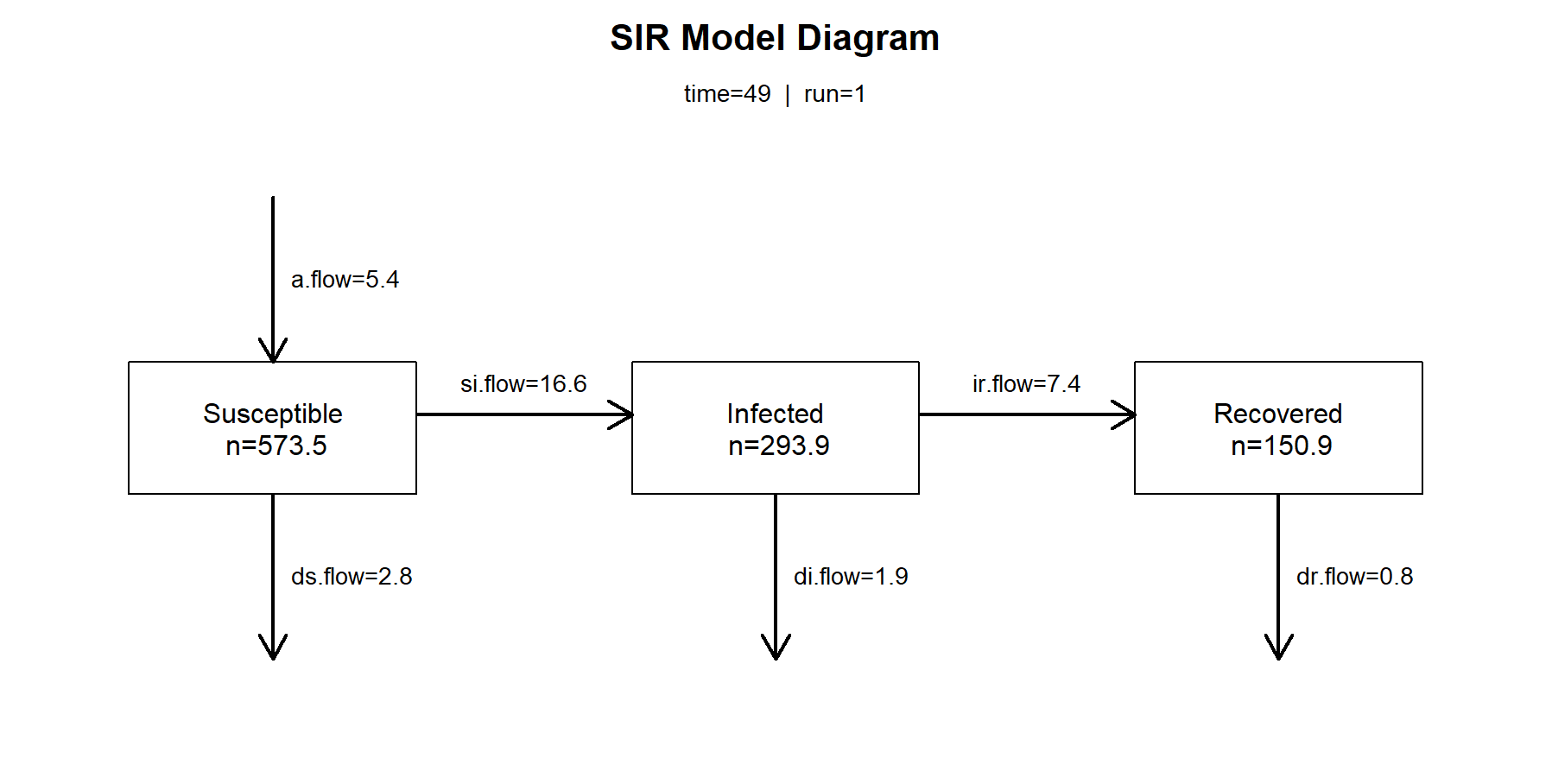
如果我们想查看在第49个观察周期的传播率数值,易感染者人数,已感染者人数,恢复者人数,以及各状态之间的传播数值。
> par(mfrow = c(1, 1))
> comp_plot(mod, at = 49, digits = 1)
查看前10条结果,和后10条结果。观察num数量,在SIR模型中,总人数增加了,因为出生率值高。
# 查看前10行
> head(as.data.frame(mod))
  time    s.num    i.num      r.num   si.flow    ir.flow   a.flow  ds.flow     di.flow       dr.flow      num
1  1.0 1000.000 1.000000 0.00000000 0.1034038 0.02587806 5.269111 5.000416 0.006469515 0.00006384888 1001.000
2  1.5 1000.165 1.071056 0.02581421 0.1107397 0.02771672 5.270491 5.001226 0.006929180 0.00019713443 1001.262
3  2.0 1000.324 1.147150 0.05333379 0.1185940 0.02968571 5.271870 5.002000 0.007421427 0.00033924715 1001.524
4  2.5 1000.475 1.228637 0.08268026 0.1270029 0.03179423 5.273250 5.002738 0.007948557 0.00049081575 1001.786
5  3.0 1000.619 1.315897 0.11398367 0.1360055 0.03405211 5.274629 5.003435 0.008513027 0.00065251323 1002.048
6  3.5 1000.754 1.409337 0.14738326 0.1456431 0.03646987 5.276008 5.004088 0.009117467 0.00082505998 1002.311

# 查看后10行
> tail(as.data.frame(mod))
     time    s.num    i.num    r.num  si.flow  ir.flow   a.flow  ds.flow   di.flow  dr.flow      num
994 497.5 348.0338 129.4081 632.5081 4.057928 3.235373 5.842185 1.740279 0.8088432 3.162722 1109.950
995 498.0 348.0778 129.4218 632.5807 4.058395 3.235716 5.842871 1.740499 0.8089290 3.163085 1110.080
996 498.5 348.1218 129.4355 632.6533 4.058862 3.236060 5.843557 1.740719 0.8090151 3.163448 1110.211
997 499.0 348.1658 129.4493 632.7260 4.059331 3.236405 5.844243 1.740939 0.8091014 3.163811 1110.341
998 499.5 348.2097 129.4631 632.7985 4.059801 3.236752 5.844930 1.741159 0.8091879 3.164174 1110.471
999 500.0 348.2537 129.4770 632.8711 4.059801 3.236752 5.844930 1.741159 0.8091879 3.164174 1110.602
4. SIS模型实现
用SIS模型进行敏感性分析,在易感-感染-恢复 (SIS) 模型中,我们在一个封闭的群体中对此进行,感染力和恢复等式相互反映,因为个体在状态之间来回流动。
建模初始:日感染率inf.prob=(0.1 0.1 0.2 0.1 0.2 0.2),日传播率 act.rate=(0.2 0.4 0.4 0.6 0.6 1),日治愈率 rec.rate=0.02。初始易感染者s.num=500,初始已感染者i.num=1,观察周期nsteps=350。
> inf<-c(0.1, 0.1, 0.2, 0.1, 0.2,0.2)
> act<-c(0.2, 0.4, 0.4, 0.6, 0.6,1)

# 设置模型传播参数
> param <- param.dcm(inf.prob = inf, act.rate = act, rec.rate = 0.02)

# 设置模型人群参数
> init <- init.dcm(s.num = 500, i.num = 1)

# 设置使用SIS模型和观察周期
> control <- control.dcm(type = "SIS", nsteps = 350)
我们同时给出了6组数据,把6组数据的参数进行微调,可一次性得出结果。运行模型,并查看模型计算结果
# 运行模型
> mod <- dcm(param, init, control)
> mod
EpiModel Simulation
=======================
Model class: dcm

Simulation Summary
-----------------------
Model type: SIS
No. runs: 6
No. time steps: 350
No. groups: 1

Model Parameters
-----------------------
inf.prob = 0.1 0.1 0.2 0.1 0.2 0.2
act.rate = 0.2 0.4 0.4 0.6 0.6 1
rec.rate = 0.02

Model Output
-----------------------
Variables: s.num i.num si.flow is.flow num
模型结果,可视化输出。同时输出6组结果,并画在一张图中,进行对比。
> par(mfrow = c(1,2), mar = c(3.2,3,2.5,1))
> plot(mod, alpha = 1, main = "Disease Prevalence",legend = "full") #已感染者数量
> plot(mod, y = "si.flow", col = "Greens", alpha = 0.8,
+      main = "Disease Incidence",legend = "full")
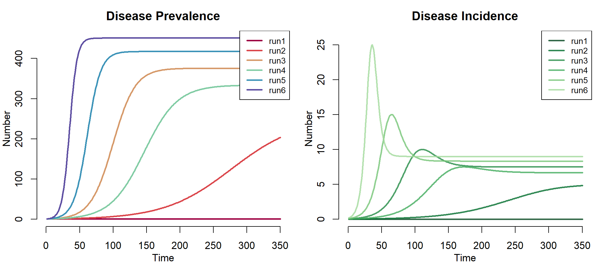
左图中,run1,run2,run3,run4,run5,run6分别表示6次运行结果,当inf.prob * act.prob 越大时,疾病从易感染者向易感染者传播越快、曲线越陡,因此run6是最高的曲线。从图中run1几乎没有传播率,是因为治愈率与传播率相等,相互低效了。右图中,为6次模拟的发病率。
SIS在计算时,根据不同的参数输入,我们共跑了6次模型,如果想查看其中某次的计算结果,可以使用run参数。
# 查看第1次运行结果的前6行输出
> head(as.data.frame(mod, run = 1)) #提取输出
  run time    s.num     i.num    si.flow    is.flow num
1   1    1 500.0000 1.0000000 0.01995968 0.01999960 501
2   1    2 500.0000 0.9999601 0.01995889 0.01999880 501
3   1    3 500.0001 0.9999202 0.01995809 0.01999800 501
4   1    4 500.0001 0.9998803 0.01995730 0.01999721 501
5   1    5 500.0002 0.9998403 0.01995650 0.01999641 501
6   1    6 500.0002 0.9998004 0.01995571 0.01999561 501

# 查看第6次运行结果的后6行输出
> tail(as.data.frame(mod, run = 6)) #提取输出
    run time s.num i.num si.flow is.flow num
345   6  345  50.1 450.9   9.018   9.018 501
346   6  346  50.1 450.9   9.018   9.018 501
347   6  347  50.1 450.9   9.018   9.018 501
348   6  348  50.1 450.9   9.018   9.018 501
349   6  349  50.1 450.9   9.018   9.018 501
350   6  350  50.1 450.9   9.018   9.018 501
5. SEIR模型实现
易感-潜伏-感染-恢复 (SEIR) 模型,扩展了 SIR 模型以包括潜伏期但非传染性的类别,模型虑了开放人群中易感人群、潜伏人群、感染者的比例。适用于存在易感者、潜伏者、患病者和康复者四类人群,有潜伏期、治愈后获得终身免疫的疾病,如带状疱疹。
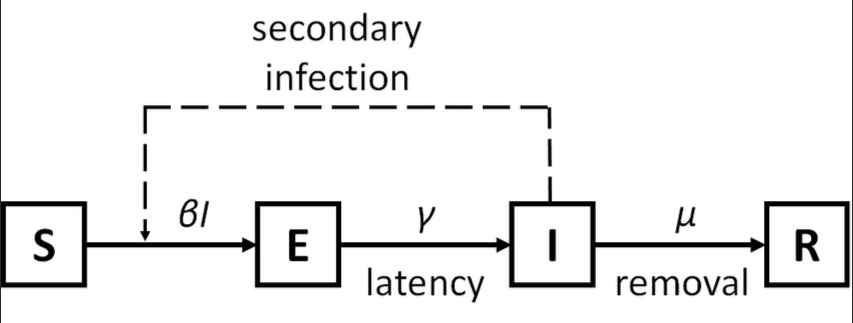
- S (Susceptible),易感染者,指缺乏免疫能力健康人,与感染者接触后容易受到感染
- E (Exposed),潜伏者 ,指接触过感染者但不存在传染性的人,可用于存在潜伏期的传染病
- I (Infectious),已感染者,指有传染性的病人,可以传播给 S,将其变为 E 或 I
- R (Recovered),康复者,指病愈后具有免疫力的人,如是终身免疫性传染病,则不可被重新变为 S 、E 或 I ,如果免疫期有限,就可以重新变为 S 类,进而被感染。
自定义SEIR模型的内核函数:
> SEIR <- function(t, t0, parms) {
+   with(as.list(c(t0, parms)), {
+
+     # Population size
+     num <- s.num + e.num + i.num + r.num
+
+     # Effective contact rate and FOI from a rearrangement of Beta * c * D
+     ce <- R0 / i.dur
+     lambda <- ce * i.num/num
+
+     dS <- -lambda*s.num
+     dE <- lambda*s.num - (1/e.dur)*e.num
+     dI <- (1/e.dur)*e.num - (1 - cfr)*(1/i.dur)*i.num - cfr*(1/i.dur)*i.num
+     dR <- (1 - cfr)*(1/i.dur)*i.num
+
+     # Compartments and flows are part of the derivative vector
+     # Other calculations to be output are outside the vector, but within the containing list
+     list(c(dS, dE, dI, dR,
+            se.flow = lambda * s.num,
+            ei.flow = (1/e.dur) * e.num,
+            ir.flow = (1 - cfr)*(1/i.dur) * i.num,
+            d.flow = cfr*(1/i.dur)*i.num),
+          num = num,
+          i.prev = i.num / num,
+          ei.prev = (e.num + i.num)/num)
+   })
+ }
建模初始:初始繁殖数R0 = 1.9, 潜伏状态的持续时间 e.dur = 10, 染状态的持续时间i.dur = 14, 病死率cfr = c(0.5, 0.7, 0.9)。初始易感染者s.num=1000*1000,初始潜伏者人数e.num=10,初始已感染者i.num=0,初始治愈者r.num=0。观察周期nsteps=350,设置自定模型函数SEIR。
# 设置模型传播参数
> param <- param.dcm(R0 = 1.9, e.dur = 10, i.dur = 14, cfr = c(0.5, 0.7, 0.9))

# 设置模型人群参数
> init <- init.dcm(s.num = 1e6, e.num = 10, i.num = 0, r.num = 0,
+                  se.flow = 0, ei.flow = 0, ir.flow = 0, d.flow = 0)

# 设置使用SEIR模型和观察周期
> control <- control.dcm(nsteps = 500, dt = 1, new.mod = SEIR)
运行模型,并查看模型计算结果
> mod <- dcm(param, init, control)
> mod
EpiModel Simulation
=======================
Model class: dcm

Simulation Summary
-----------------------
No. runs: 3
No. time steps: 500

Model Parameters
-----------------------
R0 = 1.9
e.dur = 10
i.dur = 14
cfr = 0.5 0.7 0.9

Model Output
-----------------------
Variables: s.num e.num i.num r.num se.flow ei.flow ir.flow
d.flow num i.prev ei.prev
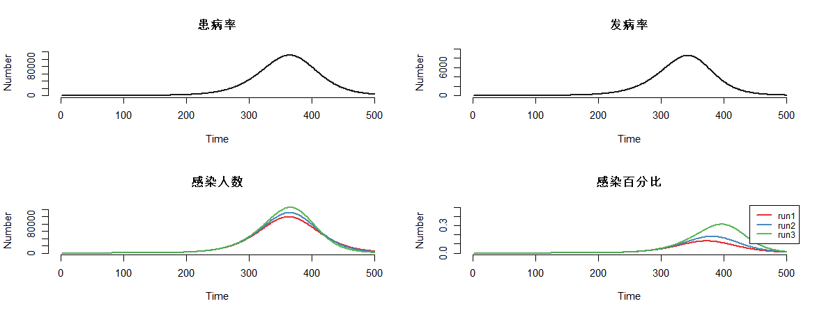
模型结果,可视化输出。通过可视化可分别描述4种状态的人群分布曲线。
par(mfrow = c(2, 2))
plot(mod, y = "i.num", run = 2, main = "患病率")
plot(mod, y = "se.flow", run = 2, main = "发病率")
plot(mod, y = "i.num", main = "感染人数")
plot(mod, y = "i.prev", main = "感染百分比", ylim = c(0, 0.5), legend = "full")
6. 基于SI模型实现组间交叉传染
EpiMoel除了能做单模型的计算,还能进行分组,做组间模型的传播实验。
我们接下来,基于SI模型实现组间交叉传播的模拟,在当前结构的两组模型中,组之间的混合纯粹是异质的:一个组只与另一组有联系,没有组内联系。
比如,在异性恋疾病传播,其中群体代表性别,我们可以将第 1 组建模为女性,将第 2 组建模为男性。
建模初始:日感染率女性inf.prob=0.4,男性inf.prob.g2=0.1。易感染者女性s.num=500男性s.num.g2=500,已感染者女性i.num=1,男性i.num.g2=0 ,观察周期nsteps=500。
# 设置模型传播参数
> param <- param.dcm(inf.prob = 0.4,  inf.prob.g2 = 0.1, act.rate = 0.25,
+ balance = "g1",a.rate = 1/100, a.rate.g2 = NA, ds.rate = 1/100,
+ ds.rate.g2 = 1/100, di.rate = 1/50, di.rate.g2 = 1/50)

# 设置模型人群参数
> init <- init.dcm(s.num = 500, i.num = 1, s.num.g2 = 500, i.num.g2 = 0)

# 设置使用SI模型和观察周期
> control <- control.dcm(type = "SI", nsteps = 500)
运行模型,并查看模型计算结果
# 运行模型
> mod <- dcm(param, init, control)
> mod
EpiModel Simulation
=======================
Model class: dcm

Simulation Summary
-----------------------
Model type: SI
No. runs: 1
No. time steps: 500
No. groups: 2

Model Parameters
-----------------------
inf.prob = 0.4
act.rate = 0.25
a.rate = 0.01
ds.rate = 0.01
di.rate = 0.02
inf.prob.g2 = 0.1
a.rate.g2 = NA
ds.rate.g2 = 0.01
di.rate.g2 = 0.02
balance = g1

Model Output
-----------------------
Variables: s.num i.num s.num.g2 i.num.g2 si.flow a.flow
ds.flow di.flow si.flow.g2 a.flow.g2 ds.flow.g2 di.flow.g2
num num.g2
模型结果,可视化输出
> par(mfrow = c(1, 1))
> plot(mod)
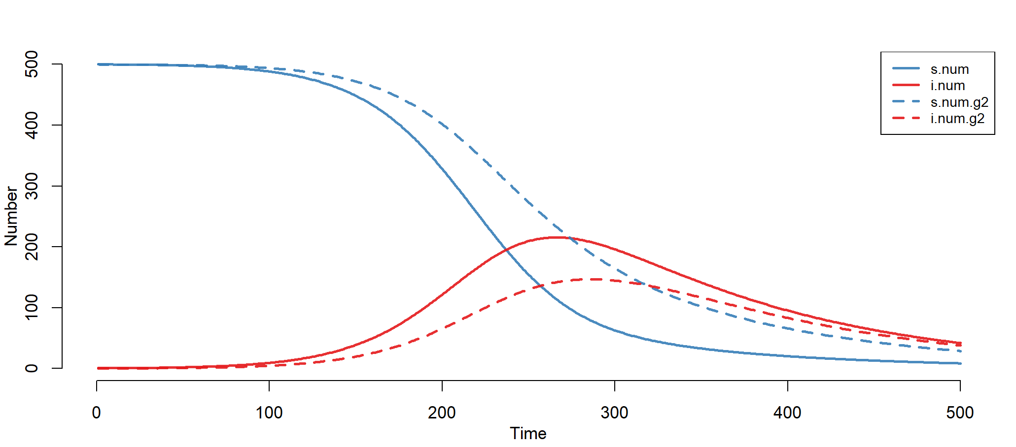
上图中,实线为女性组,虚线为男性组。
查看第20个观察周期的数据值
> summary(mod, at = 20)
EpiModel Summary
=======================
Model class: dcm

Simulation Summary
-----------------------
Model type: SI
No. runs: 1
No. time steps:
No. groups: 2

Model Statistics
------------------------------------------------------------
Time: 20	 Run: 1
------------------------------------------------------------
                   n:g1  pct:g1     n:g2  pct:g2
Suscept.        499.803   0.998  499.746   0.999
Infect.           1.016   0.002    0.376   0.001
Total           500.819   1.000  500.122   1.000
S -> I            0.038      NA    0.026      NA
Arrival ->        5.008      NA    5.008      NA
S Departure ->    4.998      NA    4.997      NA
I Departure ->    0.021      NA    0.008      NA
------------------------------------------------------------
5. 网格模型实现
使用 EpiModel 的基本网络模型,是基于时间指数随机图模型的框架构建任意复杂的联系或伙伴关系结构,这些结构会随着时间的推移而形成和消散。
官方例子:血清监测:疾病状况影响伴侣选择——人口统计过程(出生、死亡和迁移)——接触网络过程必须适应人口规模和组成的变化。对于独立模型,在每次疫情模拟开始时对全动态网络进行模拟。对于相关模型,在每个时间步长的情况下,网络被重新模拟成变化的种群大小和变化的节点属性的函数。
设置网络模型
> nw <-network.initialize(n = 1000, directed = FALSE)
> nw <-set.vertex.attribute(nw, "race", rep(0:1, each = 500))
> formation <-~edges + nodefactor("race") + nodematch("race") +concurrent
> target.stats <- c(250, 375, 225, 100)
> coef.diss <-dissolution_coefs(dissolution = ~offset(edges), duration = 25)
> est1 <- netest(nw, formation,target.stats, coef.diss, edapprox = TRUE)
Starting maximum pseudolikelihood estimation (MPLE):
Evaluating the predictor and response matrix.
Maximizing the pseudolikelihood.
Finished MPLE.
Starting Monte Carlo maximum likelihood estimation (MCMLE):
Iteration 1 of at most 60:
Optimizing with step length 1.0000.
The log-likelihood improved by 0.1944.
Estimating equations are not within tolerance region.
Iteration 2 of at most 60:
Optimizing with step length 1.0000.
The log-likelihood improved by 0.0656.
Convergence test p-value: 0.4882. Not converged with 99% confidence; increasing sample size.
Iteration 3 of at most 60:
Optimizing with step length 1.0000.
The log-likelihood improved by 0.1167.
Estimating equations are not within tolerance region.
Iteration 4 of at most 60:
Optimizing with step length 1.0000.
The log-likelihood improved by 0.0288.
Convergence test p-value: 0.0892. Not converged with 99% confidence; increasing sample size.
Iteration 5 of at most 60:
Optimizing with step length 1.0000.
The log-likelihood improved by 0.0142.
Convergence test p-value: 0.0555. Not converged with 99% confidence; increasing sample size.
Iteration 6 of at most 60:
Optimizing with step length 1.0000.
The log-likelihood improved by 0.0154.
Convergence test p-value: 0.0138. Not converged with 99% confidence; increasing sample size.
Iteration 7 of at most 60:
Optimizing with step length 1.0000.
The log-likelihood improved by 0.0047.
Convergence test p-value: 0.0002. Converged with 99% confidence.
Finished MCMLE.
This model was fit using MCMC.  To examine model diagnostics and check for degeneracy, use the
mcmc.diagnostics() function.
进行模型诊断
> #模型诊断
> dx <- netdx(est1, nsims = 5, nsteps =500,
+             nwstats.formula = ~edges + nodefactor("race", base = 0) + nodematch("race") + concurrent)

Network Diagnostics
-----------------------
- Simulating 5 networks
  |In term ‘nodefactor’ in package ‘ergm’: Argument ‘base’ has been superseded by ‘levels’, and it is recommended to use the latter.  Note that its interpretation may be different.
*****|
- Calculating formation statistics
- Calculating duration statistics
- Calculating dissolution statistics
设置模型参数
> param <- param.net(inf.prob = 0.1,act.rate = 5, rec.rate = 0.02)
> status.vector <- c(rbinom(500, 1, 0.1),rep(0, 500)) # 二项分布
> status.vector <- ifelse(status.vector ==1, "i", "s")
> init <- init.net(status.vector =status.vector)
> control <- control.net(type ="SIS", nsteps = 500, nsims = 10, epi.by = "race")
模型构建,进行各个阶段在10个周期的传播。(时间较长)
> sim1 <- netsim(est1, param, init,control)
Epidemic Simulation
----------------------------
Simulation: 10/10
Timestep: 500/500
Prevalence: 459
Population Size: 1000
----------------------------

# 查看模型运行状态和参数
> sim1
EpiModel Simulation
=======================
Model class: netsim

Simulation Summary
-----------------------
Model type: SIS
No. simulations: 10
No. time steps: 500
No. NW groups: 1

Fixed Parameters
---------------------------
inf.prob = 0.1
act.rate = 5
rec.rate = 0.02
groups = 1

Model Output
-----------------------
Variables: s.num s.num.race0 s.num.race1 i.num i.num.race0
i.num.race1 num num.race0 num.race1 si.flow is.flow
Networks: sim1 ... sim10
Transmissions: sim1 ... sim10

Formation Diagnostics
-----------------------
                  Target Sim Mean Pct Diff Sim SD
edges                250  250.084    0.034 14.896
nodefactor.race.1    375  375.007    0.002 25.379
nodematch.race       225  225.192    0.085 14.044
concurrent           100   99.629   -0.371 10.772


Dissolution Diagnostics
-----------------------
               Target Sim Mean Pct Diff Sim SD
Edge Duration   25.00   24.743   -1.026  0.295
Pct Edges Diss   0.04    0.040    0.614  0.001
查看模型运行结果
> head(as.data.frame(sim1), 10)
   sim time s.num s.num.race0 s.num.race1 i.num i.num.race0 i.num.race1  num num.race0 num.race1 si.flow is.flow
1    1    1   938         438         500    62          62           0 1000       500       500      NA      NA
2    1    2   933         434         499    67          66           1 1000       500       500       6       1
3    1    3   933         435         498    67          65           2 1000       500       500       2       2
4    1    4   933         438         495    67          62           5 1000       500       500       4       4
5    1    5   927         436         491    73          64           9 1000       500       500       7       1
6    1    6   928         438         490    72          62          10 1000       500       500       3       4
7    1    7   926         437         489    74          63          11 1000       500       500       3       1
8    1    8   924         438         486    76          62          14 1000       500       500       3       1
9    1    9   925         440         485    75          60          15 1000       500       500       2       3
10   1   10   926         440         486    74          60          14 1000       500       500       1       2
获得网络状态
# 获得网络状态
> nw <- get_network(sim1, sim = 1)

#获得每个时间点的时间状态
get_transmat(sim1, sim = 1)
画图输出2个时间点的网络状态:
> par(mfrow = c(1,2), mar = c(0,0,1,0))
> plot(sim1, type = "network", at =1, col.status = TRUE,
+      main = "Prevalence at t1")
> plot(sim1, type = "network", at =500, col.status = TRUE,
+      main = "Prevalence at t500")
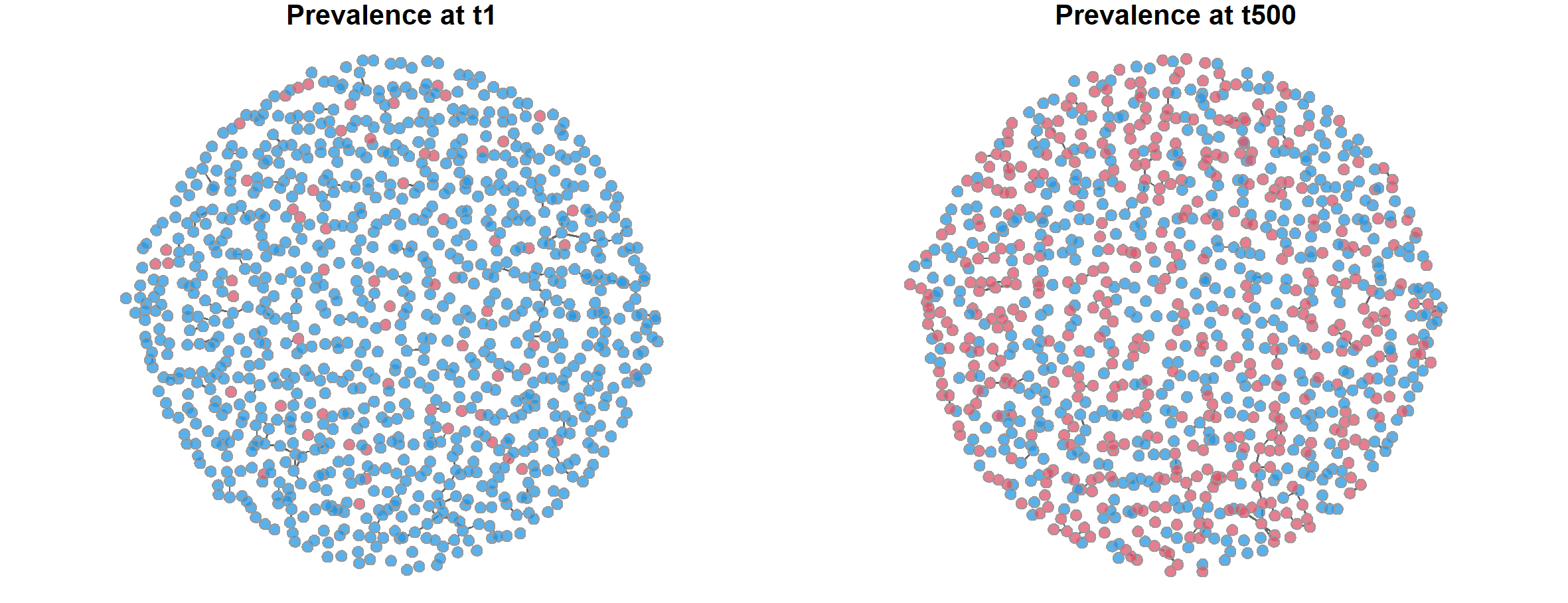
上图中左边为第1个周期的状态,右边为第500个周期的状态。
查看第500个周期的数值
> summary(sim1,at=500)

EpiModel Summary
=======================
Model class: netsim

Simulation Details
-----------------------
Model type: SIS
No. simulations: 10
No. time steps: 500
No. NW groups: 1

Model Statistics
------------------------------
Time: 500
------------------------------
            mean      sd    pct
Suscept.   529.4  13.066  0.529
Infect.    470.6  13.066  0.471
Total     1000.0   0.000  1.000
S -> I      10.8   2.821     NA
I -> S       8.5   2.915     NA
------------------------------
通过使用EpiMdoel包,让我们做传染病模型的传播模拟,快速、高效。在掌握了,传染病的基础知识后,少量的代码就可以让我们做出专业性很强的结果,确实是站在巨人的肩膀,让知识传播更快、更高效。
文本完整的代码,已经上传github,可以自由下载使用:https://github.com/bsspirit/infect/blob/main/code/model-epi.r
转载请注明出处:
http://blog.fens.me/r-epimodel