Blog Archives

R的极客理想系列文章，涵盖了R的思想，使用，工具，创新等的一系列要点，以我个人的学习和体验去诠释R的强大。

R语言作为统计学一门语言，一直在小众领域闪耀着光芒。直到大数据的爆发，R语言变成了一门炙手可热的数据分析的利器。随着越来越多的工程背景的人的加入，R语言的社区在迅速扩大成长。现在已不仅仅是统计领域，教育，银行，电商，互联网….都在使用R语言。

要成为有理想的极客，我们不能停留在语法上，要掌握牢固的数学，概率，统计知识，同时还要有创新精神，把R语言发挥到各个领域。让我们一起动起来吧，开始R的极客理想。

关于作者：

• 张丹，数据分析师/程序员/Quant: R,Java,Nodejs
• blog: http://blog.fens.me
• email: bsspirit@gmail.com

转载请注明出处：
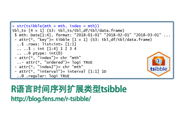
http://blog.fens.me/r-tsibble/

前言

数据科学tidyverse个项目，已经很大程度上改写的R语言的编程范式，tibble作为标准的数据结构，已替代了基础的data.frame。tsibble作为tibble对时间序列的补充，近一步规范化了数据结构，让编程更简洁。

目录

1. tsibble介绍
2. tsibble安装
3. tsibble包的基本使用

1. tsibble介绍

tsibble是一个tibble的扩展项目，用于扩展对于时间序列数据，形成一个标准化的时间序列数据结构。tibble数据类型请参考文档，R语言数据科学新类型tibble

tsibble 包提供了一个 tbl_ts 数据类，用于表示标准化的时间数据。一个 tsibble 由一个时间索引、键和其他测量变量组成，采用以数据为中心的格式，构建在 tibble 之上。

tsibble的官方网站：https://tsibble.tidyverts.org/

1.1 索引

tsibble的核心设计，就在索引的的结构。tsibble 支持广泛的索引类别：

• R 语言原生时间结构（如 Date、POSIXct 和 difftime）
• tsibble 新增的类（如 yearweek、yearmonth 和 yearquarter）
• 其他常用类：ordered、hms::hms、lubridate::period 和 nanotime::nanotime

对于具有规则间隔的 tbl_ts，需要选择索引的表示形式。例如，月度数据应使用 yearmonth 创建的时间索引，而不是 Date 或 POSIXct。因为一年中的月份确保了规律性，每年都是12个月。然而，如果使用 Date，一个月的天数在28到31天之间变化，会导致不规则的时间空间。这也适用于年-周和年-季度。

tsibble 支持任意的索引类别，只要它们能按从过去到未来的顺序排列。要支持自定义类，需要为该类定义 index_valid()，并通过 interval_pull() 计算时间间隔。

1.2 键

键变量与索引一起唯一标识每条记录：

• 空键：一个隐式变量。NULL 表示生成单变量时间序列。
• 单个变量：例如，data(pedestrian) 使用 Sensor 作为键。
• 多个变量：例如，为 data(tourism) 声明 key = c(Region, State, Purpose)。键可以与 tidy 选择器（如 starts_with()）结合使用。

1.3 时间间隔:

时间间隔:interval 函数返回与 tsibble 关联的时间间隔。

• 规则间隔：包括其值和时间单位：”nanosecond”（纳秒）、”microsecond”（微秒）、”millisecond”（毫秒）、”second”（秒）、”minute”（分）、”hour”（时）、”day”（日）、”week”（周）、”month”（月）、”quarter”（季）、”year”（年）。无法识别的时间间隔标记为 “unit”。
• 不规则间隔：as_tsibble(regular = FALSE) 生成不规则 tsibble，标记为 !。
• 未知间隔：标记为 ?，如果是空的 tsibble，或者每个键变量只有一个条目。

时间间隔基于相应的索引表示形式获得：

• “year” (Y)
• yearquarter：”quarter” (Q)
• yearmonth：”month” (M)
• yearweek：”week” (W)
• Date：”day” (D)
• difftime：”week” (W)、”day” (D)、”hour” (h)、”minute” (m)、”second” (s)
• POSIXt/hms：”hour” (h)、”minute” (m)、”second” (s)、”millisecond” (us)、”microsecond” (ms)
• period：”year” (Y)、”month” (M)、”day” (D)、”hour” (h)、”minute” (m)、”second”

(s)、”millisecond” (us)、”microsecond” (ms)

• nanotime：”nanosecond” (ns)
• 其他数值 & ordered（有序因子）：”unit”。当由于索引格式不匹配而无法获取时间间隔时，会发出错误。

时间间隔对子集操作（如 filter()、slice() 和 [.tbl_ts）保持不变。但是，如果结果是一个空的 tsibble，时间间隔总是未知的。当将 tsibble 与其他数据源连接并聚合到不同的时间尺度时，时间间隔会被重新计算。

1.4 时区

如果索引是 POSIXct，将显示索引对应的时区。? 表示获取到的时区是零长度字符 “”。

2. tsibble安装

tsibble包的安装，安装tsibble包非常简单，2条命令就可以完成，安装和加载。

# 安装
> install.packages("tsibble")

# 加载
> library(tsibble)

3. tsibble包的基本使用

3.1 构建年月日数据

构建一个tsibble数据集，“年月日”格式

# 加载时间包
> library(lubridate)

# 创建一个年月的时间
> mth <- make_date("2018") + months(0:3)
> mth
[1] "2018-01-01" "2018-02-01" "2018-03-01" "2018-04-01"

# 构造tsibble：年月日
> tsibble(mth = mth, index = mth)
# A tsibble: 4 x 1 [1D]
  mth       
      
1 2018-01-01
2 2018-02-01
3 2018-03-01
4 2018-04-01

# 构造tsibble：年月
> tsibble(mth = yearmonth(mth), index = mth)
# A tsibble: 4 x 1 [1M]
       mth
     
1 2018 1月
2 2018 2月
3 2018 3月
4 2018 4月

3.2 构建时分秒数据

构建一个tsibble数据集，“时分秒”格式。

# 构建一个时间类型，时区为shanghai
> x <- ymd_h("2015-04-05 01", tz = "Asia/Shanghai")

# 构建tsibble的时间类型
> tsibble(time = x + (c(0, 3, 6, 9)) * 60 * 60, index = time)
# A tsibble: 4 x 1 [3h] 
  time               
               
1 2015-04-05 01:00:00
2 2015-04-05 04:00:00
3 2015-04-05 07:00:00
4 2015-04-05 10:00:00

> tsibble(time = x + hours(c(0, 3, 6, 9)), index = time)
# A tsibble: 4 x 1 [3h] 
  time               
               
1 2015-04-05 01:00:00
2 2015-04-05 04:00:00
3 2015-04-05 07:00:00
4 2015-04-05 10:00:00

3.3 数据合并
分别创建数据集tsbl1为小时和数据集tsbl2为30分钟，把tsbl1和tsbl2进行合并，以小单位（30分钟）为结果输出。

> tsbl1 <- tsibble(
+   time = make_datetime(2018) + hours(0:3),
+   station = "A",
+   index = time, key = station
+ ) %>% print()
# A tsibble: 4 x 2 [1h] 
# Key:       station [1]
  time                station
                  
1 2018-01-01 00:00:00 A      
2 2018-01-01 01:00:00 A      
3 2018-01-01 02:00:00 A      
4 2018-01-01 03:00:00 A      

> tsbl2 <- tsibble(
+   time = make_datetime(2018) + minutes(seq(0, 90, by = 30)),
+   station = "B",
+   index = time, key = station
+ ) %>% print()
# A tsibble: 4 x 2 [30m] 
# Key:       station [1]
  time                station
                  
1 2018-01-01 00:00:00 B      
2 2018-01-01 00:30:00 B      
3 2018-01-01 01:00:00 B      
4 2018-01-01 01:30:00 B      

# 数据合并 
> bind_rows(tsbl1, tsbl2)
# A tsibble: 8 x 2 [30m] 
# Key:       station [2]
  time                station
                  
1 2018-01-01 00:00:00 A      
2 2018-01-01 01:00:00 A      
3 2018-01-01 02:00:00 A      
4 2018-01-01 03:00:00 A      
5 2018-01-01 00:00:00 B      
6 2018-01-01 00:30:00 B      
7 2018-01-01 01:00:00 B      
8 2018-01-01 01:30:00 B

3.4 类型转换：tibble转tsibble

把tibble转tsibble类型。

# 创建数据tibble
> x <- make_datetime(2018) + minutes(0:1)
> tbl <- tibble(  
+     time = c(x, x + minutes(15)),
+     station = rep(c("A", "B"), 2)
+ )

# 类型转换
> tbl %>% 
+     mutate(time = floor_date(time, unit = "15 mins")) %>% 
+     as_tsibble(index = time, key = station)
# A tsibble: 4 x 2 [15m] 
# Key:       station [2]
  time                station
                  
1 2018-01-01 00:00:00 A      
2 2018-01-01 00:15:00 A      
3 2018-01-01 00:00:00 B      
4 2018-01-01 00:15:00 B     

3.5 类型转换：data.frame转tsibble

data.frame转tsibble。

> df<-data.frame(
+     date=as.Date("2020-01-01")+1:1000,
+     type=sample(10,1000,replace = TRUE),
+     v1=rnorm(1000),
+     v2=runif(1000,0,1)
+ ) 

> as_tsibble(df,index = date, key = type)
# A tsibble: 1,000 x 4 [1D]
# Key:       type [10]
   date        type     v1     v2
            
 1 2020-01-20     1 -1.08  0.418 
 2 2020-02-02     1 -0.535 0.500 
 3 2020-02-05     1 -0.575 0.160 
 4 2020-02-11     1 -0.213 0.148 
 5 2020-03-02     1  0.876 0.0332
 6 2020-03-30     1  0.872 0.475 
 7 2020-04-09     1  1.05  0.539 
 8 2020-04-10     1 -1.51  0.641 
 9 2020-05-10     1 -0.630 0.632 
10 2020-06-12     1 -0.316 0.885 
# ℹ 990 more rows
# ℹ Use `print(n = ...)` to see more rows

3.6 tibble和tsibble的数据操作对比

tibble数据操作，需要定义group_by()字段。

> tbl<-tibble(df)
> tbl %>%
+   group_by(type,date) %>%
+   summarise(
+     v1_high = max(v1, na.rm = TRUE),
+     v1_low = min(v1, na.rm = TRUE)
+   )
`summarise()` has regrouped the output.
ℹ Summaries were computed grouped by type and date.
ℹ Output is grouped by type.
ℹ Use `summarise(.groups = "drop_last")` to silence this message.
ℹ Use `summarise(.by = c(type, date))` for per-operation grouping instead.
# A tibble: 1,000 × 4
# Groups:   type [10]
    type date       v1_high  v1_low
              
 1     1 2020-01-07 -0.657  -0.657 
 2     1 2020-01-15  1.87    1.87  
 3     1 2020-01-27  0.396   0.396 
 4     1 2020-01-28 -1.29   -1.29  
 5     1 2020-01-29 -1.60   -1.60  
 6     1 2020-02-12  0.825   0.825 
 7     1 2020-02-21 -0.908  -0.908 
 8     1 2020-02-28 -1.33   -1.33  
 9     1 2020-02-29  0.0145  0.0145
10     1 2020-03-06  0.177   0.177 
# ℹ 990 more rows
# ℹ Use `print(n = ...)` to see more rows

tsibble类型，通过group_by_key()，隐式地进行分组

> df_tsbl <- as_tsibble(df, key = type)
Using `date` as index variable.
> df_tsbl %>%
+   group_by_key() %>%
+   summarise(
+     v1_high = max(v1, na.rm = TRUE),
+     v1_low = min(v1, na.rm = TRUE)
+   )
# A tsibble: 1,000 x 4 [1D]
# Key:       type [10]
    type date       v1_high  v1_low
              
 1     1 2020-01-07 -0.657  -0.657 
 2     1 2020-01-15  1.87    1.87  
 3     1 2020-01-27  0.396   0.396 
 4     1 2020-01-28 -1.29   -1.29  
 5     1 2020-01-29 -1.60   -1.60  
 6     1 2020-02-12  0.825   0.825 
 7     1 2020-02-21 -0.908  -0.908 
 8     1 2020-02-28 -1.33   -1.33  
 9     1 2020-02-29  0.0145  0.0145
10     1 2020-03-06  0.177   0.177 
# ℹ 990 more rows
# ℹ Use `print(n = ...)` to see more rows

tsibble可以方便的帮助我们的整理时间类型的数据，形成干净标准的数据集，让代码看起来更数据。

转载请注明出处：
http://blog.fens.me/r-tsibble/