R的极客理想系列文章,涵盖了R的思想,使用,工具,创新等的一系列要点,以我个人的学习和体验去诠释R的强大。
R语言作为统计学一门语言,一直在小众领域闪耀着光芒。直到大数据的爆发,R语言变成了一门炙手可热的数据分析的利器。随着越来越多的工程背景的人的加入,R语言的社区在迅速扩大成长。现在已不仅仅是统计领域,教育,银行,电商,互联网….都在使用R语言。
要成为有理想的极客,我们不能停留在语法上,要掌握牢固的数学,概率,统计知识,同时还要有创新精神,把R语言发挥到各个领域。让我们一起动起来吧,开始R的极客理想。
关于作者:
- 张丹(Conan), 程序员Java,R,PHP,Javascript
- weibo:@Conan_Z
- blog: http://blog.fens.me
- email: bsspirit@gmail.com
转载请注明出处:
http://blog.fens.me/r-xts/

前言
本文是继R语言zoo时间序列基础库的扩展实现。看上去简单的时间序列,内藏复杂的规律。zoo作为时间序列的基础库,是面向通用的设计,可以用来定义股票数据,也可以分析天气数据。但由于业务行为的不同,我们需要更多的辅助函数,来帮助我们更高效的完成任务。
xts扩展了zoo,提供更多的数据处理和数据变换的函数。
目录
- xts介绍
- xts安装
- xts数据结构
- xts的API介绍
- xts使用
1. xts介绍
xts是对时间序列数据(zoo)的一种扩展实现,目标是为了统一时间序列的操作接口。实际上,xts类型继承了zoo类型,丰富了时间序列数据处理的函数,API定义更贴近使用者,更实用,更简单!
xts项目地址:http://r-forge.r-project.org/projects/xts/
2. xts安装
系统环境
- Win7 64bit
- R: 3.0.1 x86_64-w64-mingw32/x64 b4bit
xts安装
> install.packages("xts")
also installing the dependency ‘zoo’

trying URL 'http://mirror.bjtu.edu.cn/cran/bin/windows/contrib/3.0/zoo_1.7-10.zip'
Content type 'application/zip' length 875046 bytes (854 Kb)
opened URL
downloaded 854 Kb

trying URL 'http://mirror.bjtu.edu.cn/cran/bin/windows/contrib/3.0/xts_0.9-7.zip'
Content type 'application/zip' length 661664 bytes (646 Kb)
opened URL
downloaded 646 Kb

package ‘zoo’ successfully unpacked and MD5 sums checked
package ‘xts’ successfully unpacked and MD5 sums checked
3. xts数据结构
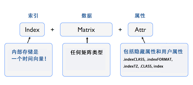
xts扩展zoo的基础结构,由3部分组合。
- 索引部分:时间类型向量
- 数据部分:以矩阵为基础类型,支持可以与矩阵相互转换的任何类型
- 属性部分:附件信息,包括时区,索引时间类型的格式等
4. xts的API介绍
xts基础
- xts: 定义xts数据类型,继承zoo类型
- coredata.xts: 对xts部分数据赋值
- xtsAttributes: xts对象属性赋值
- [.xts: 用[]语法,取数据子集
- dimnames.xts: xts维度名赋值
- sample_matrix: 测试数据集,包括180条xts对象的记录,matrix类型
- xtsAPI: C语言API接口
类型转换
- as.xts: 转换对象到xts(zoo)类型
- as.xts.methods: 转换对象到xts函数
- plot.xts: 为plot函数,提供xts的接口作图
- .parseISO8601: 把字符串(ISO8601格式)输出为,POSIXct类型的,包括开始时间和结束时间的list对象
- firstof: 创建一个开始时间,POSIXct类型
- lastof: 创建一个结束时间,POSIXct类型
- indexClass: 取索引类型
- .indexDate: 取索引的
- .indexday: 索引的日值
- .indexyday: 索引的年(日)值
- .indexmday: 索引的月(日)值
- .indexwday: 索引的周(日)值
- .indexweek: 索引的周值
- .indexmon: 索引的月值
- .indexyear: 索引的年值
- .indexhour: 索引的时值
- .indexmin: 索引的分值
- .indexsec: 索引的秒值
数据处理
- align.time: 以下一个时间对齐数据,秒,分钟,小时
- endpoints: 按时间单元提取索引数据
- merge.xts: 合并多个xts对象,重写zoo::merge.zoo函数
- rbind.xts: 数据按行合并,为rbind函数,提供xts的接口
- split.xts: 数据分隔,为split函数,提供xts的接口
- na.locf.xts: 替换NA值,重写zoo:na.locf函数
数据统计
- apply.daily: 按日分割数据,执行函数
- apply.weekly: 按周分割数据,执行函数
- apply.monthly: 按月分割数据,执行函数
- apply.quarterly: 按季分割数据,执行函数
- apply.yearly: 按年分割数据,执行函数
- to.period: 按期间分割数据
- period.apply: 按期间执行自定义函数
- period.max: 按期间计算最大值
- period.min: 按期间计算最小值
- period.prod: 按期间计算指数
- period.sum: 按期间求和
- nseconds: 计算数据集,包括多少秒
- nminutes: 计算数据集,包括多少分
- nhours: 计算数据集,包括多少时
- ndays: 计算数据集,包括多少日
- nweeks: 计算数据集,包括多少周
- nmonths: 计算数据集,包括多少月
- nquarters: 计算数据集,包括多少季
- nyears: 计算数据集,包括多少年
- periodicity: 查看时间序列的期间
辅助工具
- first: 从开始到结束,设置条件取子集
- last: 从结束到开始,设置条件取子集
- timeBased: 判断是否是时间类型
- timeBasedSeq: 创建时间的序列
- diff.xts: 计算步长和差分
- isOrdered: 检查向量是否是顺序的
- make.index.unique: 强制时间唯一,增加毫秒随机数
- axTicksByTime: 计算X轴刻度标记位置按时间描述
- indexTZ: 查询xts对象的时区
5. xts使用
- 1). xts类型基本操作
- 2). xts的作图
- 3). xts类型转换
- 4). xts数据处理
- 5). xts数据统计计算
- 6). xts时间序列工具使用
1). xts类型基本操作
测试数据集sample_matrix
> library(xts)
> data(sample_matrix)
> head(sample_matrix)
               Open     High      Low    Close
2007-01-02 50.03978 50.11778 49.95041 50.11778
2007-01-03 50.23050 50.42188 50.23050 50.39767
2007-01-04 50.42096 50.42096 50.26414 50.33236
2007-01-05 50.37347 50.37347 50.22103 50.33459
2007-01-06 50.24433 50.24433 50.11121 50.18112
2007-01-07 50.13211 50.21561 49.99185 49.99185
定义xts类型对象
> sample.xts <- as.xts(sample_matrix, descr='my new xts object')
> class(sample.xts)
[1] "xts" "zoo"

> str(sample.xts)
An ‘xts’ object on 2007-01-02/2007-06-30 containing:
  Data: num [1:180, 1:4] 50 50.2 50.4 50.4 50.2 ...
 - attr(*, "dimnames")=List of 2
  ..$ : NULL
  ..$ : chr [1:4] "Open" "High" "Low" "Close"
  Indexed by objects of class: [POSIXct,POSIXt] TZ:
  xts Attributes:
List of 1
 $ descr: chr "my new xts object"

> head(sample.xts)
               Open     High      Low    Close
2007-01-02 50.03978 50.11778 49.95041 50.11778
2007-01-03 50.23050 50.42188 50.23050 50.39767
2007-01-04 50.42096 50.42096 50.26414 50.33236
2007-01-05 50.37347 50.37347 50.22103 50.33459
2007-01-06 50.24433 50.24433 50.11121 50.18112
2007-01-07 50.13211 50.21561 49.99185 49.99185

> attr(sample.xts,'descr')
[1] "my new xts object"
xts数据查询
> head(sample.xts['2007'])
               Open     High      Low    Close
2007-01-02 50.03978 50.11778 49.95041 50.11778
2007-01-03 50.23050 50.42188 50.23050 50.39767
2007-01-04 50.42096 50.42096 50.26414 50.33236
2007-01-05 50.37347 50.37347 50.22103 50.33459
2007-01-06 50.24433 50.24433 50.11121 50.18112
2007-01-07 50.13211 50.21561 49.99185 49.99185

> head(sample.xts['2007-03/'])
               Open     High      Low    Close
2007-03-01 50.81620 50.81620 50.56451 50.57075
2007-03-02 50.60980 50.72061 50.50808 50.61559
2007-03-03 50.73241 50.73241 50.40929 50.41033
2007-03-04 50.39273 50.40881 50.24922 50.32636
2007-03-05 50.26501 50.34050 50.26501 50.29567
2007-03-06 50.27464 50.32019 50.16380 50.16380

> head(sample.xts['2007-03-06/2007'])
               Open     High      Low    Close
2007-03-06 50.27464 50.32019 50.16380 50.16380
2007-03-07 50.14458 50.20278 49.91381 49.91381
2007-03-08 49.93149 50.00364 49.84893 49.91839
2007-03-09 49.92377 49.92377 49.74242 49.80712
2007-03-10 49.79370 49.88984 49.70385 49.88698
2007-03-11 49.83062 49.88295 49.76031 49.78806

> sample.xts['2007-01-03']
              Open     High     Low    Close
2007-01-03 50.2305 50.42188 50.2305 50.39767
2). 操作xts的作图
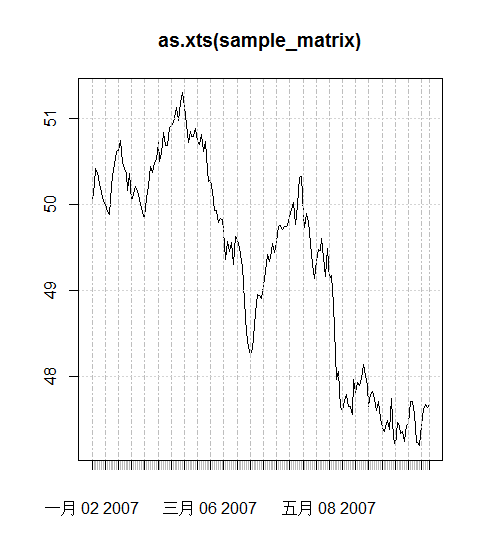
曲线图
> data(sample_matrix)
> plot(sample_matrix)

> plot(as.xts(sample_matrix))
Warning message:
In plot.xts(as.xts(sample_matrix)) :
  only the univariate series will be plotted
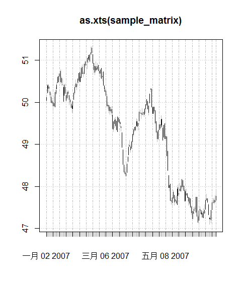
K线图
> plot(as.xts(sample_matrix), type='candles')
3). xts类型转换
分别创建首尾时间:firstof, lastof
> firstof(2000)
[1] "2000-01-01 CST"

> firstof(2005,01,01)
[1] "2005-01-01 CST"

> lastof(2007)
[1] "2007-12-31 23:59:59.99998 CST"

> lastof(2007,10)
[1] "2007-10-31 23:59:59.99998 CST"
创建首尾时间
> .parseISO8601('2000')
$first.time
[1] "2000-01-01 CST"

$last.time
[1] "2000-12-31 23:59:59.99998 CST"

> .parseISO8601('2000-05/2001-02')
$first.time
[1] "2000-05-01 CST"

$last.time
[1] "2001-02-28 23:59:59.99998 CST"

> .parseISO8601('2000-01/02')
$first.time
[1] "2000-01-01 CST"

$last.time
[1] "2000-02-29 23:59:59.99998 CST"

> .parseISO8601('T08:30/T15:00')
$first.time
[1] "1970-01-01 08:30:00 CST"

$last.time
[1] "1970-12-31 15:00:59.99999 CST"
取索引类型
> x <- timeBasedSeq('2010-01-01/2010-01-02 12:00')
> x <- xts(1:length(x), x)

> head(x)
                    [,1]
2010-01-01 00:00:00    1
2010-01-01 00:01:00    2
2010-01-01 00:02:00    3
2010-01-01 00:03:00    4
2010-01-01 00:04:00    5
2010-01-01 00:05:00    6

> indexClass(x)
[1] "POSIXt"  "POSIXct"
索引时间格式化
> indexFormat(x) <- "%Y-%b-%d %H:%M:%OS3"
> head(x)
                          [,1]
2010-一月-01 00:00:00.000    1
2010-一月-01 00:01:00.000    2
2010-一月-01 00:02:00.000    3
2010-一月-01 00:03:00.000    4
2010-一月-01 00:04:00.000    5
2010-一月-01 00:05:00.000    6
取索引时间
> .indexhour(head(x))
[1] 0 0 0 0 0 0

> .indexmin(head(x))
[1] 0 1 2 3 4 5
4). xts数据处理
数据对齐
> x <- Sys.time() + 1:30

#整10秒对齐
> align.time(x, 10)
 [1] "2013-11-18 15:42:30 CST" "2013-11-18 15:42:30 CST"
 [3] "2013-11-18 15:42:30 CST" "2013-11-18 15:42:40 CST"
 [5] "2013-11-18 15:42:40 CST" "2013-11-18 15:42:40 CST"
 [7] "2013-11-18 15:42:40 CST" "2013-11-18 15:42:40 CST"
 [9] "2013-11-18 15:42:40 CST" "2013-11-18 15:42:40 CST"
[11] "2013-11-18 15:42:40 CST" "2013-11-18 15:42:40 CST"
[13] "2013-11-18 15:42:40 CST" "2013-11-18 15:42:50 CST"
[15] "2013-11-18 15:42:50 CST" "2013-11-18 15:42:50 CST"
[17] "2013-11-18 15:42:50 CST" "2013-11-18 15:42:50 CST"
[19] "2013-11-18 15:42:50 CST" "2013-11-18 15:42:50 CST"
[21] "2013-11-18 15:42:50 CST" "2013-11-18 15:42:50 CST"
[23] "2013-11-18 15:42:50 CST" "2013-11-18 15:43:00 CST"
[25] "2013-11-18 15:43:00 CST" "2013-11-18 15:43:00 CST"
[27] "2013-11-18 15:43:00 CST" "2013-11-18 15:43:00 CST"
[29] "2013-11-18 15:43:00 CST" "2013-11-18 15:43:00 CST"

#整60秒对齐
> align.time(x, 60)
 [1] "2013-11-18 15:43:00 CST" "2013-11-18 15:43:00 CST"
 [3] "2013-11-18 15:43:00 CST" "2013-11-18 15:43:00 CST"
 [5] "2013-11-18 15:43:00 CST" "2013-11-18 15:43:00 CST"
 [7] "2013-11-18 15:43:00 CST" "2013-11-18 15:43:00 CST"
 [9] "2013-11-18 15:43:00 CST" "2013-11-18 15:43:00 CST"
[11] "2013-11-18 15:43:00 CST" "2013-11-18 15:43:00 CST"
[13] "2013-11-18 15:43:00 CST" "2013-11-18 15:43:00 CST"
[15] "2013-11-18 15:43:00 CST" "2013-11-18 15:43:00 CST"
[17] "2013-11-18 15:43:00 CST" "2013-11-18 15:43:00 CST"
[19] "2013-11-18 15:43:00 CST" "2013-11-18 15:43:00 CST"
[21] "2013-11-18 15:43:00 CST" "2013-11-18 15:43:00 CST"
[23] "2013-11-18 15:43:00 CST" "2013-11-18 15:43:00 CST"
[25] "2013-11-18 15:43:00 CST" "2013-11-18 15:43:00 CST"
[27] "2013-11-18 15:43:00 CST" "2013-11-18 15:43:00 CST"
[29] "2013-11-18 15:43:00 CST" "2013-11-18 15:43:00 CST"
按时间分割数据,并计算
> xts.ts <- xts(rnorm(231),as.Date(13514:13744,origin="1970-01-01"))
> apply.monthly(xts.ts,mean)
                  [,1]
2007-01-31  0.17699984
2007-02-28  0.30734220
2007-03-31 -0.08757189
2007-04-30  0.18734688
2007-05-31  0.04496954
2007-06-30  0.06884836
2007-07-31  0.25081814
2007-08-19 -0.28845938

> apply.monthly(xts.ts,function(x) var(x))
                [,1]
2007-01-31 0.9533217
2007-02-28 0.9158947
2007-03-31 1.2821450
2007-04-30 1.2805976
2007-05-31 0.9725438
2007-06-30 1.5228904
2007-07-31 0.8737030
2007-08-19 0.8490521

> apply.quarterly(xts.ts,mean)
                 [,1]
2007-03-31 0.12642053
2007-06-30 0.09977926
2007-08-19 0.04589268

> apply.yearly(xts.ts,mean)
                 [,1]
2007-08-19 0.09849522
按期间分隔:to.period
> data(sample_matrix)
> to.period(sample_matrix)
           sample_matrix.Open sample_matrix.High sample_matrix.Low sample_matrix.Close
2007-01-31           50.03978           50.77336          49.76308            50.22578
2007-02-28           50.22448           51.32342          50.19101            50.77091
2007-03-31           50.81620           50.81620          48.23648            48.97490
2007-04-30           48.94407           50.33781          48.80962            49.33974
2007-05-31           49.34572           49.69097          47.51796            47.73780
2007-06-30           47.74432           47.94127          47.09144            47.76719
> class(to.period(sample_matrix))
[1] "matrix"

> samplexts <- as.xts(sample_matrix)
> to.period(samplexts)
           samplexts.Open samplexts.High samplexts.Low samplexts.Close
2007-01-31       50.03978       50.77336      49.76308        50.22578
2007-02-28       50.22448       51.32342      50.19101        50.77091
2007-03-31       50.81620       50.81620      48.23648        48.97490
2007-04-30       48.94407       50.33781      48.80962        49.33974
2007-05-31       49.34572       49.69097      47.51796        47.73780
2007-06-30       47.74432       47.94127      47.09144        47.76719
> class(to.period(samplexts))
[1] "xts" "zoo"
按期间分割索引数据
> data(sample_matrix)

> endpoints(sample_matrix)
[1]   0  30  58  89 119 150 180

> endpoints(sample_matrix, 'days',k=7)
 [1]   0   6  13  20  27  34  41  48  55  62  69  76  83  90  97 104 111 118 125
[20] 132 139 146 153 160 167 174 180

> endpoints(sample_matrix, 'weeks')
 [1]   0   7  14  21  28  35  42  49  56  63  70  77  84  91  98 105 112 119 126
[20] 133 140 147 154 161 168 175 180

> endpoints(sample_matrix, 'months')
[1]   0  30  58  89 119 150 180
数据合并:按列合并
> (x <- xts(4:10, Sys.Date()+4:10))
           [,1]
2013-11-22    4
2013-11-23    5
2013-11-24    6
2013-11-25    7
2013-11-26    8
2013-11-27    9
2013-11-28   10

> (y <- xts(1:6, Sys.Date()+1:6))
           [,1]
2013-11-19    1
2013-11-20    2
2013-11-21    3
2013-11-22    4
2013-11-23    5
2013-11-24    6

> merge(x,y)
            x  y
2013-11-19 NA  1
2013-11-20 NA  2
2013-11-21 NA  3
2013-11-22  4  4
2013-11-23  5  5
2013-11-24  6  6
2013-11-25  7 NA
2013-11-26  8 NA
2013-11-27  9 NA
2013-11-28 10 NA

#取索引将领合并
> merge(x,y, join='inner')
           x y
2013-11-22 4 4
2013-11-23 5 5
2013-11-24 6 6

#以左侧为基础合并
> merge(x,y, join='left')
            x  y
2013-11-22  4  4
2013-11-23  5  5
2013-11-24  6  6
2013-11-25  7 NA
2013-11-26  8 NA
2013-11-27  9 NA
2013-11-28 10 NA
数据合并:按行合并
> x <- xts(1:3, Sys.Date()+1:3)

> rbind(x,x)
           [,1]
2013-11-19    1
2013-11-19    1
2013-11-20    2
2013-11-20    2
2013-11-21    3
2013-11-21    3
数据切片:按行切片
> data(sample_matrix)
> x <- as.xts(sample_matrix)

按月切片
> split(x)[[1]]
               Open     High      Low    Close
2007-01-02 50.03978 50.11778 49.95041 50.11778
2007-01-03 50.23050 50.42188 50.23050 50.39767
2007-01-04 50.42096 50.42096 50.26414 50.33236
2007-01-05 50.37347 50.37347 50.22103 50.33459
2007-01-06 50.24433 50.24433 50.11121 50.18112
2007-01-07 50.13211 50.21561 49.99185 49.99185
2007-01-08 50.03555 50.10363 49.96971 49.98806
2007-01-09 49.99489 49.99489 49.80454 49.91333
2007-01-10 49.91228 50.13053 49.91228 49.97246
2007-01-11 49.88529 50.23910 49.88529 50.23910
2007-01-12 50.21258 50.35980 50.17176 50.28519
2007-01-13 50.32385 50.48000 50.32385 50.41286
2007-01-14 50.46359 50.62395 50.46359 50.60145
2007-01-15 50.61724 50.68583 50.47359 50.48912
2007-01-16 50.62024 50.73731 50.56627 50.67835
2007-01-17 50.74150 50.77336 50.44932 50.48644
2007-01-18 50.48051 50.60712 50.40269 50.57632
2007-01-19 50.41381 50.55627 50.41278 50.41278
2007-01-20 50.35323 50.35323 50.02142 50.02142
2007-01-21 50.16188 50.42090 50.16044 50.42090
2007-01-22 50.36008 50.43875 50.21129 50.21129
2007-01-23 50.03966 50.16961 50.03670 50.16961
2007-01-24 50.10953 50.26942 50.06387 50.23145
2007-01-25 50.20738 50.28268 50.12913 50.24334
2007-01-26 50.16008 50.16008 49.94052 50.07024
2007-01-27 50.06041 50.09777 49.97267 50.01091
2007-01-28 49.96586 50.00217 49.87468 49.88096
2007-01-29 49.85624 49.93038 49.76308 49.91875
2007-01-30 49.85477 50.02180 49.77242 50.02180
2007-01-31 50.07049 50.22578 50.07049 50.22578

按周切片
> split(x, f="weeks")[[1]]
               Open     High      Low    Close
2007-01-02 50.03978 50.11778 49.95041 50.11778
2007-01-03 50.23050 50.42188 50.23050 50.39767
2007-01-04 50.42096 50.42096 50.26414 50.33236
2007-01-05 50.37347 50.37347 50.22103 50.33459
2007-01-06 50.24433 50.24433 50.11121 50.18112
2007-01-07 50.13211 50.21561 49.99185 49.99185
2007-01-08 50.03555 50.10363 49.96971 49.98806
> split(x, f="weeks")[[2]]
               Open     High      Low    Close
2007-01-09 49.99489 49.99489 49.80454 49.91333
2007-01-10 49.91228 50.13053 49.91228 49.97246
2007-01-11 49.88529 50.23910 49.88529 50.23910
2007-01-12 50.21258 50.35980 50.17176 50.28519
2007-01-13 50.32385 50.48000 50.32385 50.41286
2007-01-14 50.46359 50.62395 50.46359 50.60145
2007-01-15 50.61724 50.68583 50.47359 50.48912
NA值处理
> x <- xts(1:10, Sys.Date()+1:10)
> x[c(1,2,5,9,10)] <- NA
> x
           [,1]
2013-11-19   NA
2013-11-20   NA
2013-11-21    3
2013-11-22    4
2013-11-23   NA
2013-11-24    6
2013-11-25    7
2013-11-26    8
2013-11-27   NA
2013-11-28   NA

#取前一个
> na.locf(x)
           [,1]
2013-11-19   NA
2013-11-20   NA
2013-11-21    3
2013-11-22    4
2013-11-23    4
2013-11-24    6
2013-11-25    7
2013-11-26    8
2013-11-27    8
2013-11-28    8

#取后一个
> na.locf(x, fromLast=TRUE)
           [,1]
2013-11-19    3
2013-11-20    3
2013-11-21    3
2013-11-22    4
2013-11-23    6
2013-11-24    6
2013-11-25    7
2013-11-26    8
2013-11-27   NA
2013-11-28   NA
5). xts数据统计计算
取开始时间,结束时间
> xts.ts <- xts(rnorm(231),as.Date(13514:13744,origin="1970-01-01"))

> start(xts.ts)
[1] "2007-01-01"
> end(xts.ts)
[1] "2007-08-19"

> periodicity(xts.ts)
Daily periodicity from 2007-01-01 to 2007-08-19
计算时间区间
> data(sample_matrix)
> ndays(sample_matrix)
[1] 180
> nweeks(sample_matrix)
[1] 26
> nmonths(sample_matrix)
[1] 6
> nquarters(sample_matrix)
[1] 2
> nyears(sample_matrix)
[1] 1
按期间计算统计指标
> zoo.data <- zoo(rnorm(31)+10,as.Date(13514:13744,origin="1970-01-01"))

#按周获得期间
> ep <- endpoints(zoo.data,'weeks')
> ep
 [1]   0   7  14  21  28  35  42  49  56  63  70  77  84  91  98 105 112 119
[19] 126 133 140 147 154 161 168 175 182 189 196 203 210 217 224 231

#计算周的均值
> period.apply(zoo.data, INDEX=ep, FUN=function(x) mean(x))
2007-01-07 2007-01-14 2007-01-21 2007-01-28 2007-02-04 2007-02-11 2007-02-18
 10.200488   9.649387  10.304151   9.864847  10.382943   9.660175   9.857894
2007-02-25 2007-03-04 2007-03-11 2007-03-18 2007-03-25 2007-04-01 2007-04-08
 10.495037   9.569531  10.292899   9.651616  10.089103   9.961048  10.304860
2007-04-15 2007-04-22 2007-04-29 2007-05-06 2007-05-13 2007-05-20 2007-05-27
  9.658432   9.887531  10.608082   9.747787  10.052955   9.625730  10.430030
2007-06-03 2007-06-10 2007-06-17 2007-06-24 2007-07-01 2007-07-08 2007-07-15
  9.814703  10.224869   9.509881  10.187905  10.229310  10.261725   9.855776
2007-07-22 2007-07-29 2007-08-05 2007-08-12 2007-08-19
  9.445072  10.482020   9.844531  10.200488   9.649387

#计算周的最大值
> head(period.max(zoo.data, INDEX=ep))
               [,1]
2007-01-07 12.05912
2007-01-14 10.79286
2007-01-21 11.60658
2007-01-28 11.63455
2007-02-04 12.05912
2007-02-11 10.67887

#计算周的最小值
> head(period.min(zoo.data, INDEX=ep))
               [,1]
2007-01-07 8.874509
2007-01-14 8.534655
2007-01-21 9.069773
2007-01-28 8.461555
2007-02-04 9.421085
2007-02-11 8.534655

#计算周的一个指数值
> head(period.prod(zoo.data, INDEX=ep))
               [,1]
2007-01-07 11140398
2007-01-14  7582350
2007-01-21 11930334
2007-01-28  8658933
2007-02-04 12702505
2007-02-11  7702767
6). xts时间序列工具使用
检查时间类型
> timeBased(Sys.time())
[1] TRUE
> timeBased(Sys.Date())
[1] TRUE
> timeBased(200701)
[1] FALSE
创建时间序列
#按年
> timeBasedSeq('1999/2008')
 [1] "1999-01-01" "2000-01-01" "2001-01-01" "2002-01-01" "2003-01-01"
 [6] "2004-01-01" "2005-01-01" "2006-01-01" "2007-01-01" "2008-01-01"

#按月
> head(timeBasedSeq('199901/2008'))
[1] "十二月 1998" "一月 1999"   "二月 1999"   "三月 1999"   "四月 1999"
[6] "五月 1999"

#按日
> head(timeBasedSeq('199901/2008/d'),40)
 [1] "十二月 1998" "一月 1999"   "一月 1999"   "一月 1999"   "一月 1999"
 [6] "一月 1999"   "一月 1999"   "一月 1999"   "一月 1999"   "一月 1999"
[11] "一月 1999"   "一月 1999"   "一月 1999"   "一月 1999"   "一月 1999"
[16] "一月 1999"   "一月 1999"   "一月 1999"   "一月 1999"   "一月 1999"
[21] "一月 1999"   "一月 1999"   "一月 1999"   "一月 1999"   "一月 1999"
[26] "一月 1999"   "一月 1999"   "一月 1999"   "一月 1999"   "一月 1999"
[31] "一月 1999"   "一月 1999"   "二月 1999"   "二月 1999"   "二月 1999"
[36] "二月 1999"   "二月 1999"   "二月 1999"   "二月 1999"   "二月 1999"

#按数量创建,100分钟的数据集
> timeBasedSeq('20080101 0830',length=100)
$from
[1] "2008-01-01 08:30:00 CST"
$to
[1] NA
$by
[1] "mins"
$length.out
[1] 100
按索引取数据first, last
> x <- xts(1:100, Sys.Date()+1:100)

> head(x)
           [,1]
2013-11-19    1
2013-11-20    2
2013-11-21    3
2013-11-22    4
2013-11-23    5
2013-11-24    6

> first(x, 10)
           [,1]
2013-11-19    1
2013-11-20    2
2013-11-21    3
2013-11-22    4
2013-11-23    5
2013-11-24    6
2013-11-25    7
2013-11-26    8
2013-11-27    9
2013-11-28   10

> first(x, '1 day')
           [,1]
2013-11-19    1

> last(x, '1 weeks')
           [,1]
2014-02-24   98
2014-02-25   99
2014-02-26  100
计算步长和差分
> x <- xts(1:5, Sys.Date()+1:5)
#正向
> lag(x)
           [,1]
2013-11-19   NA
2013-11-20    1
2013-11-21    2
2013-11-22    3
2013-11-23    4

#反向
> lag(x, k=-1, na.pad=FALSE)
           [,1]
2013-11-19    2
2013-11-20    3
2013-11-21    4
2013-11-22    5

#1阶差分
> diff(x)
           [,1]
2013-11-19   NA
2013-11-20    1
2013-11-21    1
2013-11-22    1
2013-11-23    1

#2阶差分
> diff(x, lag=2)
           [,1]
2013-11-19   NA
2013-11-20   NA
2013-11-21    2
2013-11-22    2
2013-11-23    2
检查向量是否排序好的
> isOrdered(1:10, increasing=TRUE)
[1] TRUE

> isOrdered(1:10, increasing=FALSE)
[1] FALSE

> isOrdered(c(1,1:10), increasing=TRUE)
[1] FALSE

> isOrdered(c(1,1:10), increasing=TRUE, strictly=FALSE)
[1] TRUE
强制唯一索引
> x <- xts(1:5, as.POSIXct("2011-01-21") + c(1,1,1,2,3)/1e3)
> x
                        [,1]
2011-01-21 00:00:00.000    1
2011-01-21 00:00:00.000    2
2011-01-21 00:00:00.000    3
2011-01-21 00:00:00.002    4
2011-01-21 00:00:00.003    5

> make.index.unique(x)
                           [,1]
2011-01-21 00:00:00.000999    1
2011-01-21 00:00:00.001000    2
2011-01-21 00:00:00.001001    3
2011-01-21 00:00:00.002000    4
2011-01-21 00:00:00.003000    5
查询xts对象时区
> x <- xts(1:10, Sys.Date()+1:10)

> indexTZ(x)
[1] "UTC"
> tzone(x)
[1] "UTC"

> str(x)
An ‘xts’ object on 2013-11-19/2013-11-28 containing:
  Data: int [1:10, 1] 1 2 3 4 5 6 7 8 9 10
  Indexed by objects of class: [Date] TZ: UTC
  xts Attributes:
 NULL
xts给了zoo类型时间序列更多的API支持,这样我们就有了更方便的工具,可以做各种的时间序列的转换和变形了。
转载请注明出处:
http://blog.fens.me/r-xts/

R太强大,一个xts就够看一段时间
xts也是基础类型,很多地方都能用上。
请问一下是否能够实现把多个xts对象放在一个集合中(每个对象类似于向量中的元素),通过索引来引用这些元素呢?
可以,自己构造一个这样的类型就行了。
谢谢您的回复!我是利用getsymbols从雅虎获取多支股票的数据,每支股票的信息都储存在s[i]中,用哪些命令可以构造一个s集合,然后再利用循环给s中的元素赋值呢?
s[[i]], If you want to work with elements in lists, you use [[]] when you want to change the list itself, you use [].
因为一个个地命令输入来获得股票的数据太麻烦了!我想将需要的股票的代码构造为一个向量,利用循环来自动搜索这些股票代码的数据,但是不知道定义下述的集合s。非常冒昧地打扰您了,还请不吝赐教!
> stock for(i in seq(stock))
+ {
+ s[i]<-getSymbols(stock[i],from = "2011-05-01",to = "2014-05-01",auto.assign=FALSE)
+ }
就是不知道如何定义上述代码中的s
你把s定义为list类型吧,容易扩展一点。
如下代码思路:
s<-list()
for(){
s[i]<-getSymbols(stock[i],from = "2011-05-01",to = "2014-05-01",auto.assign=FALSE)
}
列表我有尝试过,但是不行!不知道您所说的扩展指什么?
s<-list()
stock<-c("600016.ss","600059.ss","600060.ss","600069.ss")
for(i in stock){
s[i]<-getSymbols(i,from = "2011-05-01",to = "2014-05-01",auto.assign=FALSE)
}
s
> s stock for(i in seq(stock))
+ {
+ s[i]<-getSymbols(stock[i],from="2011-05-01",to="2014-05-01",auto.assign=FALSE)
+ }
Warning messages:
1: In s[i] <- getSymbols(stock[i], from = "2011-05-01", to = "2014-05-01", :
number of items to replace is not a multiple of replacement length
2: In s[i] <- getSymbols(stock[i], from = "2011-05-01", to = "2014-05-01", :
number of items to replace is not a multiple of replacement length
3: In s[i] <- getSymbols(stock[i], from = "2011-05-01", to = "2014-05-01", :
number of items to replace is not a multiple of replacement length
4: In s[i] s
[[1]]
[1] 6.11
[[2]]
[1] 11.83
[[3]]
[1] 14.61
[[4]]
[1] 11.28
得到的s[i]中只有一个数据
翻看了《R语言编程艺术》,我知道您的意思了,您是要我使用S3类进行定义,谢谢您了!
您好,不好意思,又要打扰您。上面的这个问题我确实无法解决,这个似乎是要预先定义一个类似于C#中的集合类,但是对于用R语言做这件事情确实无从下手。不知道您是否能够提供一个具体的思考方向,在此感激不尽!
一门编程语言要从头学起,不能用一下学一下,这样永远自己解决不了问题。去Dataguru.cn报个R的入门班学吧。
[…] R语言本身提供了丰富的金融函数工具包,quantmod包就是最常用的一个,另外还要配合时间序列包zoo和xts,指标计算包TTR,可视包ggplot2等一起使用。关于zoo包和xts包的详细使用可以参考文章R语言时间序列基础库zoo,可扩展的时间序列xts。 […]
[…] R语言本身提供了丰富的金融函数工具包,时间序列包zoo和xts,指标计算包TTR,数据处理包plyr,可视包ggplot2等,我们会一起使用这些工具包来完成建模、计算和可视化的工作。关于zoo包和xts包的详细使用可以参考文章,R语言时间序列基础库zoo,可扩展的时间序列xts。 […]
[…] R语言本身提供了丰富的金融函数工具包,时间序列包zoo和xts,指标计算包TTR,数据处理包plyr,可视包ggplot2等,我们会一起使用这些工具包来完成建模、计算和可视化的工作。关于zoo包和xts包的详细使用可以参考文章,R语言时间序列基础库zoo,可扩展的时间序列xts。 […]
[…] 关于xts包的介绍,请参考文章:可扩展的时间序列xts […]
[…] 除了R语言的内置基础数据类型,对于金融的数据处理,一般我会把它变成标准的时间序列类型的数据,R语言中基本的时间序列的类型为 zoo 和 xts类型,当然还有一些其他包提供的数据类型。关于zoo和xts的详细介绍,请参考文章 R语言时间序列基础库zoo,可扩展的时间序列xts […]